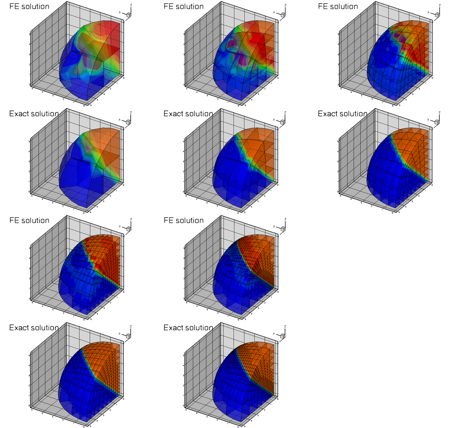
Following the numerous 2D problems discussed in earlier examples we now demonstrate that the solution of 3D problems is just as easy. For this purpose we discuss the adaptive solution of the 3D Poisson problem
 , with Dirichlet boundary conditions , with Dirichlet boundary conditions
 is given. is given. |
We choose a source function and boundary conditions for which
![\[ u_0(x_1,x_2,x_3) = \tanh\left(1-\alpha(({\bf x}-{\bf x_0}) \cdot {\bf N})\right), \ \ \ \ \ \ \ \ \ (3) \]](form_4.png)
is the exact solution. Here where  is the vector of the spatial coordinates, and the vectors
  and
and  are constants. For large values of the constant
  the solution varies rapidly across the plane through
  whose normal is given by
  .
.
Here are some plots of the exact and computed solutions for  ,
,  , and
, and  at various levels of mesh refinement. Note that the plot of the exact solution was produced by setting the nodal values to the exact solution, obtained by evaluating (3) at the nodal positions. The elements' basis functions were then used to interpolate between the nodal values. On the coarse meshes, the interpolation between the "exact" nodal values is clearly inadequate to resolve the rapid variation of the solution.

Global parameters and functions
Following our usual practice, we use a namespace, TanhSolnForPoisson, to define the source function, the exact solution and various problem parameters.
The driver code
The driver code solves the 3D Poisson problem with full spatial adaptivity – a fairly time-consuming process. To minimise the run-times when the code is executed during oomph-lib's self-tests, we use command line arguments to optionally limit the number of adaptive refinements. If the code is run with a(ny) command line arguments, only a single adaptive refinement is performed; otherwise up to four levels of refinement are permitted. oomph-lib provides storage for the command line arguments in the namespace CommandLineArgs to make them accessible to other parts of the code.
Otherwise the driver code is very similar to that used in the corresponding 2D Poisson problems: We construct the problem, passing the pointer to the source function. Next, we create a DocInfo object to specify the output directory, and execute the global self-test to assert that the problem has been set up correctly. Next we solve the problem on the coarse initial mesh (comprising four 27-node brick elements) and then adapt the problem based on the elemental error estimates, until the maximum number of adaptations has been reached or until the adaptation ceases to changes the mesh.
The problem class
The problem class has the usual structure – the only difference to the corresponding 2D codes is that the assignment of the boundary conditions in actions_before_newton_solve() now involves thee nodal coordinates rather than two.
[See the discussion of the 1D Poisson problem for a more detailed discussion of the function type PoissonEquations<3>::PoissonSourceFctPt.]
The Problem constructor
In the Problem constructor, we set the "steepness parameter"  to a large value and create the mesh for a a sphere of radius 5. Next, we create the error estimator and pass it to the adaptive mesh.
We adjust the targets for the mesh adaptation so that the single mesh adaptation performed during a validation run produces a non-uniform refinement pattern. (The error targets for this case were determined by trial and error.) The tighter error tolerances specified otherwise are appropriate to properly resolve the solution, as shown in the animated gif files at the beginning of this document.
Next, we assign the boundary conditions. In the present problem all boundaries are Dirichlet boundaries, therefore we loop over all nodes on all boundaries and pin their values. If only a subset of the mesh boundaries were of Dirichlet type, only the nodes on those boundaries would have to be pinned. "Usually" the numbering of the mesh boundaries is (or at least should be!) documented in the mesh constructor but it can also be obtained from the function Mesh::output_boundaries(...) whose use is illustrated here.
Finally we loop over all elements to assign the source function pointer, and then call the generic Problem::assign_eqn_numbers() routine to set up the equation numbers.
Post-processing
The function doc_solution(...) writes the FE solution and the corresponding exact solution, defined in TanhSolnForPoisson::get_exact_u(...) to disk. The DocInfo object specifies the output directory and the label for the file names. [See the discussion of the 1D Poisson problem for a more detailed discussion of the generic Mesh member functions Mesh::output(...), Mesh::output_fct(...) and Mesh::compute_error(...)].
Source files for this tutorial
- The source files for this tutorial are located in the directory:
demo_drivers/poisson/eighth_sphere_poisson/ - The driver code is:
demo_drivers/poisson/eighth_sphere_poisson/eighth_sphere_poisson.cc
PDF file
A pdf version of this document is available.
![\[ \sum_{i=1}^3 \frac{\partial^2u}{\partial x_i^2} = f(x_1,x_2,x_3), \ \ \ \ \ \ \ \ \ \ (1) \]](form_0.png)
![\[ \left. u\right|_{\partial D}=u_0 \ \ \ \ \ \ \ \ \ \ (2) \]](form_2.png)