The problem of steady flow in a curved tube is considered with a prescribed Poiseuille flow at the inlet and a traction-free outlet condition. It is not clear that the latter is appropriate, but the main aim of this example is to check that the TubeMesh works correctly.
A detailed comparison between the flow field and the Dean solution should be performed for validation purposes, but the qualitative features seem reasonable.
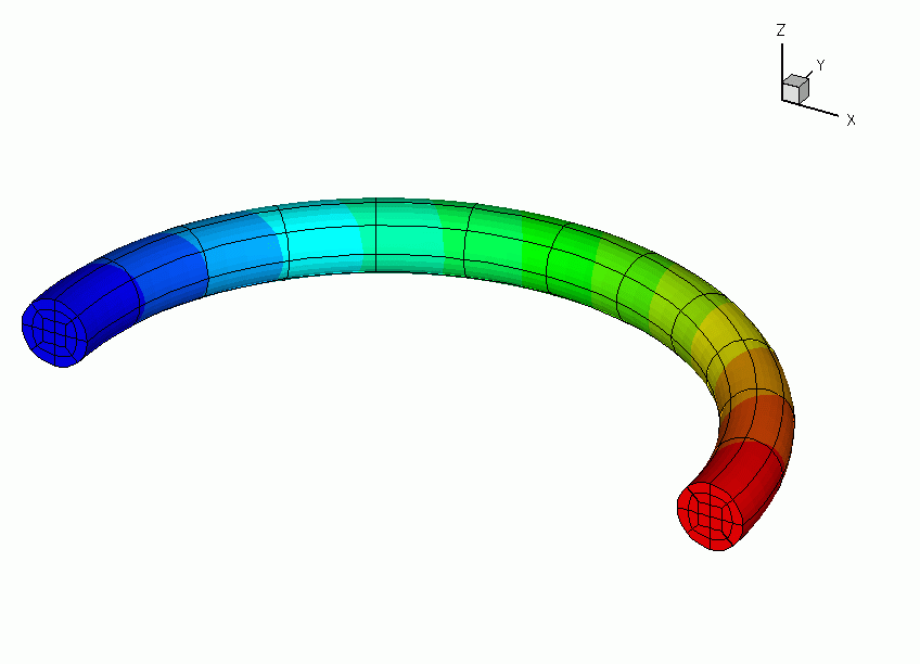
Sketch of the problem with pressure contours.
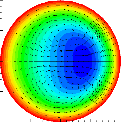
Contours of axial velocity and secondary streamlines.
Detailed documentation to be written. Here's the driver code...
//LIC// ====================================================================
//LIC// This file forms part of oomph-lib, the object-oriented,
//LIC// multi-physics finite-element library, available
//LIC// at http://www.oomph-lib.org.
//LIC//
//LIC// Version 1.0; svn revision $LastChangedRevision$
//LIC//
//LIC// $LastChangedDate$
//LIC//
//LIC// Copyright (C) 2006-2016 Matthias Heil and Andrew Hazel
//LIC//
//LIC// This library is free software; you can redistribute it and/or
//LIC// modify it under the terms of the GNU Lesser General Public
//LIC// License as published by the Free Software Foundation; either
//LIC// version 2.1 of the License, or (at your option) any later version.
//LIC//
//LIC// This library is distributed in the hope that it will be useful,
//LIC// but WITHOUT ANY WARRANTY; without even the implied warranty of
//LIC// MERCHANTABILITY or FITNESS FOR A PARTICULAR PURPOSE. See the GNU
//LIC// Lesser General Public License for more details.
//LIC//
//LIC// You should have received a copy of the GNU Lesser General Public
//LIC// License along with this library; if not, write to the Free Software
//LIC// Foundation, Inc., 51 Franklin Street, Fifth Floor, Boston, MA
//LIC// 02110-1301 USA.
//LIC//
//LIC// The authors may be contacted at oomph-lib@maths.man.ac.uk.
//LIC//
//LIC//====================================================================
///Driver for a 3D navier stokes steady entry flow problem in a
///uniformly curved tube
//Generic routines
#include "generic.h"
#include "navier_stokes.h"
// The mesh
#include "meshes/tube_mesh.h"
using namespace std;
using namespace oomph;
//=start_of_MyCurvedCylinder===================================
//A geometric object that represents the geometry of the domain
//================================================================
{
public:
/// Constructor that takes the radius and curvature of the tube
/// as its arguments
GeomObject(3,3), Radius(radius), Delta(delta) { }
/// Destructor
virtual~MyCurvedCylinder(){}
///Lagrangian coordinate xi
void position (const Vector<double>& xi, Vector<double>& r) const
{
r[0] = (1.0/Delta)*cos(xi[0]) + xi[2]*Radius*cos(xi[0])*cos(xi[1]);
r[1] = (1.0/Delta)*sin(xi[0]) + xi[2]*Radius*sin(xi[0])*cos(xi[1]);
r[2] = -xi[2]*Radius*sin(xi[1]);
}
/// Return the position of the tube as a function of time
/// (doesn't move as a function of time)
void position(const unsigned& t,
const Vector<double>& xi, Vector<double>& r) const
{
position(xi,r);
}
private:
///Storage for the radius of the tube
double Radius;
//Storage for the curvature of the tube
double Delta;
};
//=start_of_namespace================================================
/// Namespace for physical parameters
//===================================================================
namespace Global_Physical_Variables
{
/// Reynolds number
double Re=50;
/// The desired curvature of the pipe
double Delta=0.1;
} // end_of_namespace
//=start_of_problem_class=============================================
/// Entry flow problem in tapered tube domain
//====================================================================
template<class ELEMENT>
{
public:
/// Constructor: Pass DocInfo object and target errors
const double& max_error_target);
/// Destructor (empty)
~SteadyCurvedTubeProblem() {}
/// \short Update the problem specs before solve
void actions_before_newton_solve();
/// After adaptation: Pin redudant pressure dofs.
void actions_after_adapt()
{
// Pin redudant pressure dofs
RefineableNavierStokesEquations<3>::
pin_redundant_nodal_pressures(mesh_pt()->element_pt());
}
/// Doc the solution
void doc_solution();
/// \short Overload generic access function by one that returns
/// a pointer to the specific mesh
RefineableTubeMesh<ELEMENT>* mesh_pt()
{
return dynamic_cast<RefineableTubeMesh<ELEMENT>*>(Problem::mesh_pt());
}
private:
/// Doc info object
DocInfo Doc_info;
///Pointer to GeomObject that specifies the domain volume
GeomObject *Volume_pt;
}; // end_of_problem_class
//=start_of_constructor===================================================
/// Constructor: Pass DocInfo object and error targets
//========================================================================
template<class ELEMENT>
SteadyCurvedTubeProblem<ELEMENT>::SteadyCurvedTubeProblem(DocInfo& doc_info,
const double& min_error_target,
const double& max_error_target)
: Doc_info(doc_info)
{
// Setup mesh:
//------------
// Create GeomObject that specifies the domain geometry
//The radius of the tube is one and the curvature is specified by
//the global variable Delta.
//Define pi
const double pi = MathematicalConstants::Pi;
//Set the centerline coordinates spanning the mesh
Vector<double> centreline_limits(2);
centreline_limits[0] = 0.0;
centreline_limits[1] = pi;
//Set the positions of the angles that divide the outer ring
//These must be in the range -pi,pi, ordered from smallest to
//largest
Vector<double> theta_positions(4);
theta_positions[0] = -0.75*pi;
theta_positions[1] = -0.25*pi;
theta_positions[2] = 0.25*pi;
theta_positions[3] = 0.75*pi;
//Define the radial fraction of the central box (always halfway
//along the radius)
Vector<double> radial_frac(4,0.5);
// Number of layers in the initial mesh
unsigned nlayer=6;
// Build and assign mesh
Problem::mesh_pt()= new RefineableTubeMesh<ELEMENT>(Volume_pt,
centreline_limits,
theta_positions,
radial_frac,
nlayer);
// Set error estimator
Z2ErrorEstimator* error_estimator_pt=new Z2ErrorEstimator;
mesh_pt()->spatial_error_estimator_pt()=error_estimator_pt;
// Error targets for adaptive refinement
mesh_pt()->max_permitted_error()=max_error_target;
mesh_pt()->min_permitted_error()=min_error_target;
// Set the boundary conditions for this problem: All nodal values are
// free by default -- just pin the ones that have Dirichlet conditions
// here.
//Choose the conventional form by setting gamma to zero
//The boundary conditions will be pseudo-traction free (d/dn = 0)
ELEMENT::Gamma[0] = 0.0;
ELEMENT::Gamma[1] = 0.0;
ELEMENT::Gamma[2] = 0.0;
//Loop over the boundaries
unsigned num_bound = mesh_pt()->nboundary();
for(unsigned ibound=0;ibound<num_bound;ibound++)
{
unsigned num_nod= mesh_pt()->nboundary_node(ibound);
for (unsigned inod=0;inod<num_nod;inod++)
{
// Boundary 0 is the inlet symmetry boundary:
// Boundary 1 is the tube wall
// Pin all values
if((ibound==0) || (ibound==1))
{
mesh_pt()->boundary_node_pt(ibound,inod)->pin(0);
mesh_pt()->boundary_node_pt(ibound,inod)->pin(1);
mesh_pt()->boundary_node_pt(ibound,inod)->pin(2);
}
}
} // end loop over boundaries
// Loop over the elements to set up element-specific
// things that cannot be handled by constructor
unsigned n_element = mesh_pt()->nelement();
for(unsigned i=0;i<n_element;i++)
{
// Upcast from GeneralisedElement to the present element
ELEMENT* el_pt = dynamic_cast<ELEMENT*>(mesh_pt()->element_pt(i));
//Set the Reynolds number, etc
el_pt->re_pt() = &Global_Physical_Variables::Re;
}
// Pin redudant pressure dofs
RefineableNavierStokesEquations<3>::
pin_redundant_nodal_pressures(mesh_pt()->element_pt());
//Attach the boundary conditions to the mesh
cout <<"Number of equations: " << assign_eqn_numbers() << std::endl;
} // end_of_constructor
//=start_of_actions_before_newton_solve===================================
/// Set the inflow boundary conditions
//========================================================================
template<class ELEMENT>
{
// (Re-)assign velocity profile at inflow values
//--------------------------------------------
unsigned ibound=0;
unsigned num_nod= mesh_pt()->nboundary_node(ibound);
for (unsigned inod=0;inod<num_nod;inod++)
{
// Recover coordinates of tube relative to centre position
double x=mesh_pt()->boundary_node_pt(ibound,inod)->x(0) -
double z=mesh_pt()->boundary_node_pt(ibound,inod)->x(2);
//Calculate the radius
double r=sqrt(x*x+z*z);
// Poiseuille-type profile for axial velocity (component 1 at the inlet)
mesh_pt()->boundary_node_pt(ibound,inod)->
set_value(1,(1.0-pow(r,2.0)));
}
} // end_of_actions_before_newton_solve
//=start_of_doc_solution==================================================
/// Doc the solution
//========================================================================
template<class ELEMENT>
{
//Output file stream
ofstream some_file;
char filename[100];
// Number of plot points
unsigned npts;
npts=5;
//Need high precision for large radii of curvature
//some_file.precision(10);
// Output solution labelled by the Reynolds number
sprintf(filename,"%s/soln_Re%g.dat",Doc_info.directory().c_str(),
some_file.open(filename);
mesh_pt()->output(some_file,npts);
some_file.close();
} // end_of_doc_solution
////////////////////////////////////////////////////////////////////////
////////////////////////////////////////////////////////////////////////
////////////////////////////////////////////////////////////////////////
//=start_of_main=======================================================
/// Driver for 3D entry flow into a curved tube. If there are
/// any command line arguments, we regard this as a validation run
/// and perform only a single adaptation
//=====================================================================
{
// Store command line arguments
CommandLineArgs::setup(argc,argv);
// Allow (up to) two rounds of fully automatic adapation in response to
//-----------------------------------------------------------------------
// error estimate
//---------------
unsigned max_adapt;
double max_error_target,min_error_target;
// Set max number of adaptations in black-box Newton solver and
// error targets for adaptation
if (CommandLineArgs::Argc==1)
{
// Up to two adaptations
max_adapt=2;
// Error targets for adaptive refinement
max_error_target=0.001;
min_error_target=0.00001;
}
// Validation run: Only one adaptation. Relax error targets
// for faster solution
else
{
// Validation run: Just one round of adaptation
max_adapt=1;
// Error targets for adaptive refinement
max_error_target=0.02;
min_error_target=0.002;
}
// end max_adapt setup
// Set up doc info
DocInfo doc_info;
// Do Taylor-Hood elements
//------------------------
{
// Set output directory
doc_info.set_directory("RESLT_TH");
// Step number
doc_info.number()=0;
// Build problem
problem(doc_info,min_error_target,max_error_target);
cout << " Doing Taylor-Hood elements " << std::endl;
// Solve the problem
problem.newton_solve(max_adapt);
// Doc solution after solving
problem.doc_solution();
}
// Do Crouzeix-Raviart elements
//------------------------
{
// Set output directory
doc_info.set_directory("RESLT_CR");
// Step number
doc_info.number()=0;
// Build problem
problem(doc_info,min_error_target,max_error_target);
cout << " Doing Crouzeix-Raviart elements " << std::endl;
// Solve the problem
problem.newton_solve(max_adapt);
// Doc solution after solving
problem.doc_solution();
}
} // end_of_main
PDF file
A pdf version of this document is available.